This is a test
Contact
MCM Alchimia premium license certificate
Alchimia software
To get your premium license please visit our premium launching page or use paypal button in MCM Alchimia application
With your 1 year premium licence you will be able to print GUM framework uncertainty budget (new in version 4), export and save output Monte Carlo simulation samples as a .csv file, export and save output chart as .jpg graphic file and export and save a frequency histogram (w/ 100 intervals ) from Monte Carlo simulation results.
Your saved models will be operative after upgrade. Please, let us know whichever problem with MCM Alchimia premium to support@mcm-alchimia.com.
To activate premium version click on “ugrade to premium” small button on left side of the application, below menu buttons panel. Next, in upgrade panel, copy small and long key codes from this certificate and paste them on corresponding text fields. Finally click on “Check premium codes” button.
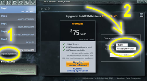
Upgrade to MCM Alchimia 4 premium (1 year licence)
For most of your lab applications we trust MCM Alchimia free version is enough, and surely you will agree that this is the best, easiest and most featured application for uncertainty estimation. However, this project is under permanent improvement and research with the generous help and knowledge of engineers, laboratory technicians, developers, statisticians, and university students. This effort is obviously not free in time nor money for us. Thus, we reserve some features for experts, researchers and enterprises in a premium version.
With this small support you will be helping to keep most of our MCM Alchimia free for all.
With your 1 year premium licence you will be able to:
- Print GUM framework uncertainty budget (new in version 4).
- Export and save output Monte Carlo simulation samples as a .csv file
- Export and save output chart as .jpg graphic file.
- Export and save a frequency histogram (w/ 100 intervals ) from Monte Carlo simulation results.
Functions REG_x (y) and REG_y (x)
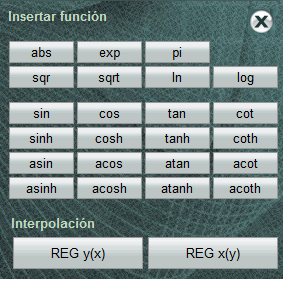 To open the function keyboard, click on the f (x) link that is located on the equation editor when we position ourselves on it.
In the lower section of the function keyboard, there are two interpolation buttons that allow you to obtain linear interpolation results in the connected curve. These generic variables perform not only the interpolation in the curve but also perform the uncertainty estimation of it, integrating its contribution to the model.
It is important to understand that this calculation does not represent what is usually done when we do it manually, but it integrates all the tools available in the simulation of the model, as well as the data obtained during the simulation of the connected curve.
REG_y (x). Interpolates the observed response ( y ) of an indicated value from x axis, estimating its associated total uncertainty. The value of x can be numerical, a variable or even part of the model equation. For example REG_y (5), REG_y (A) or REG_y (coef_a * ABS (A1-A2)).
REG_x (y). Given a value, variable or fragment of the equation corresponding to y axis, interpolate and estimate the associated uncertainty of the corresponding value of x .
Uncertainty of interpolation.
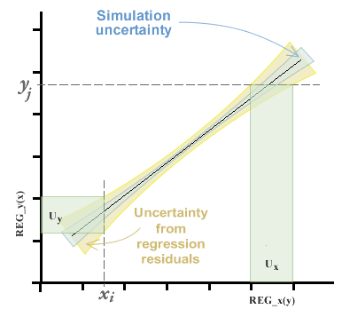
In the chapter on Using the calibration curve panel we saw that we could estimate the curve of best fit by the method of ordinary, inverse and total least squares (the latter by means of the method of analysis of the primary component). Whichever method is chosen, we will obtain coefficients of the equation of the line, in addition to a range of variable uncertainty along the curve, composed of the uncertainty of simulation and that contributed by the variance of the residuals. This topic can be seen in more depth in the chapter of regressions and curves .
The uncertainty in the interpolation, then, will be given by the standard error of the curve in the axis from which it intends to interpolate.
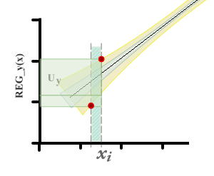
It can be seen that there are two differences with respect to the method that is usually used to estimate uncertainty in calibration curves. First, zero uncertainty is not expected on the x axis.
On the other hand, when you want to estimate the value of x i from a y i observed, the uncertainty interval in x is taken from the residual variance in x . In the graphs you can see a representation of the uncertainty of the measurand in each case.
Using regressions panel
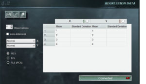 The regression panel of MCM Infinite Alchimia allows great flexibility when constructing a calibration curve for our test model.
Panel Features
1. Menu buttons In the upper left section of the panel there are three buttons that are unique to this panel.
![]() Save. Allows you to save the data entered for the curve. This data is saved independently of the model. In this way you can use the same curve in other models and, conversely, use other calibration curves in the same model when necessary. The curves will be saved with extension .mcr.
Save. Allows you to save the data entered for the curve. This data is saved independently of the model. In this way you can use the same curve in other models and, conversely, use other calibration curves in the same model when necessary. The curves will be saved with extension .mcr.
![]()
Open curve. This button allows you to open a previously saved MCM Alchimia curve. Opening a curve does not imply that it is connected, so after opening it, you must press the connect button so that it is connected.
![]() Clear data. Deletes all the data entered in the panel.
Clear data. Deletes all the data entered in the panel.
& nbsp;
2. Number of observations. Using the forward and back buttons, the number of observations we will use to define the curve can be modified. The software offers 5 by default, but an unlimited number of observation can be indicated with a minimum of 3.
3. Intercept with zero. Selecting this option will result in an independent term = 0, regardless of the input values. In certain situations, this restriction can be defined by the knowledge of the process, for which this option is available.
4. Distribution menu. In the upper right corner of this panel are the drop-down menus where we can select probability distributions, both for the independent term, and for the dependent one. The distributions available in these combos are: Constant, Rectangular, Triangular and Normal.
If you select Constant, you are assuming that the entries on that axis have no uncertainty so the property column will be inactive and data can not be entered. In other cases, the standard deviation should be defined for the case of the normal distribution or the semi-interval for the rectangular or triangular.
5. Data panel. In this field you enter the average values of x and y , as well as the properties of the distribution we choose for each axis. Important! This panel allows you to copy and paste data from any worksheet with the same form. If the copied range has larger dimensions than those indicated in the data panel, the remaining data will be truncated. The cell selected in the panel will be the upper-left cell of the copied range.
In the title cell of each axis there is a check box. Pressing this box the data of the first row of data of that axis will be copied in all the following rows.
6. Minimal square selector. In this selector we select the type of least squares method that will be used to obtain the calibration curve.
- OLS. Ordinary Least Squares. The curve obtained through this method will be the one for which the quadratic sum of the residuals in y is minimal.
- ILS. Inverse Least Squares. The curve obtained through this method will be the one for which the quadratic sum of the residuals in x is minimal.
- TLS (PCA). Total Least Squares. The curve obtained through this method will be the one for which the quadratic sum of the orthogonal residuals to the curve is minimal.

Regressions and calibration curves
Important : This article, and therefore, the use of the tool for curves of MCM Alchimia does not take into account the assumptions related to the application of Least Squares, such as normality, linearity, homoscedasticity, and independence. The study and validation of these assumptions allow us to know the quality and applicability of the linear representation from the input data, however MCM Alchimia, allows to connect curves constructed from any input data set performing unplaced least squares and does not ensure or control compliance with these assumptions.
It is common to find trials, analytical methods or calibrations that are based on the measurement at different levels of the analyte or in different positions of the reading scale, when it is an instrument. In this way, in most cases a linear relation between them is considered, obtaining by the least squares method the coefficients of the equation of the line: ![]()
In this way when it comes to equipment calibration and the correction is plotted according to the reading scale, it is easy to obtain this value by applying the equation above, from the coefficients obtained by least squares and the reading.
But it is also usual especially in the area of chemistry to construct the calibration curve with certified reference materials of known concentration and then use this curve to obtain the concentration of an analyte from an observed response.

In the least squares analysis we have three types of uncertainty associated with the curve.
- Random errors in reference responses yi.
- Random effects on reference values xi .
- Effect associated with the presumption of linearity, which will be given by the waste.
If the values xi and yi do not present uncertainty, the curve obtained will be the one that minimizes the squares of the waste. In case of random errors in reference values xi and yi are greater than zero, it is possible to generate pseudo-randomizations with the distribution associated to each parameter, obtaining by least squares a curve for each data set. This generates an additional uncertainty in the regression coefficients, in addition to the uncertainty determined by the residuals.
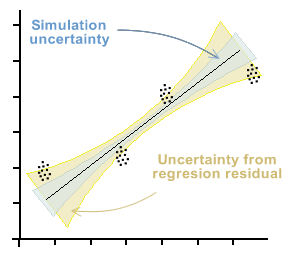
In the graph below, the beam of points that each observation would represent if there is a significant uncertainty in both axes is presented symbolically. This situation therefore yields a bundle of curves that satisfy the least squares of the residuals, generating uncertainty in both regression coefficients. This uncertainty is marked with blue in the graph.
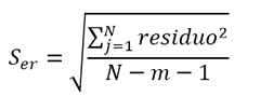
Furthermore, this uncertainty will be increased by the uncertainty inherent in the curve, which is determined as a function of the standard deviation of the residual errors. This uncertainty, in general, is greater than that of the simulation and is represented by the orange zone in the graph.
What does MCM Alchimia software do when connecting a curve?
After all the values are entered into the panel, in order to use the curve in our model, we must “connect” the curve with the button provided for that purpose. When we do this, MCM Alchimia performs a simulation with the data set, performing a random sampling with the input data and the response. For each of the iterations, the regression coefficients b 0 and b 1 are obtained, and a value of the coefficient of determination R 2 .
As in the traditional simulation, a population of data for these parameters with unknown distribution is obtained, and will depend on the distributions and values of the input data.
In order not to make assumptions or inadequate approximations about these statistical properties, MCM Alchimia keeps the set of values in vectors associated with these random variables, which will be available throughout the process.
On the other hand, with the average values of each pair of input data, the application calculates the uncertainty of the curve, as a function of the regression residuals.
This repository of sampling data will be used according to the need of our model, either to use the coefficients b0 and b1 with their uncertainty, to consider the uncertainty of the curve or to use the interpolation functions that will be described later.
Correlated variables
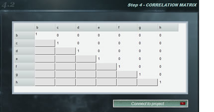 Frequently test models are used that contain two or more magnitudes with some degree of correlation, that is, that systematically, when modifying the value of one of them, the other increases or decreases. The correlation coefficients between two variables vary between -1 and 1, where the value indicates the strength of the correlation, while the sign indicates the direction. In this way, we understand that if the correlation is = 1 there is an absolute direct proportionality between the magnitudes whereas if the value is -1 the proportionality is inverse. On the other hand, a zero value for the correlation coefficient indicates that the variables are independent.
If we know the correlation coefficients between the magnitudes of the mathematical model of our trial we can use the correlation panel. The correlation matrix is automatically constructed with the variables of our model so that we indicate the correlation coefficient between them. When we complete the matrix, click on the < connect to the project > and after checking that the matrix is correct, the green light of the button will indicate that it is connected.
In this case, the simulation will be done with correlated variables. If at any time we want to work with independent magnitudes again, we only have to uncheck the checkbox < correlated > on the simulation button. In this way we can alternate between both states without correcting the correlation matrix each time.
Regression
NOTE: This tool is only available for models with connected curves (See work with curves)

At the end of the list of distributions, MCM Alchimia have available this tool that allows to assign regression parameters to our test model. In this way, we have 3 options related to our connected curve to choose from:
- B0. Independent coefficient (ordinate at the origin) of the connected curve.
- B1. Coefficient of the first order of the connected curve.
Both B0 and B1 will have associated uncertainties that correspond to the result of the simulation, that is, if at least one of the values used to construct the curve had uncertainty, the simulation will necessarily produce a succession of curves for each set of simulated values, each with coefficients B0 and B1 that will have some degree of variation. The magnitude of this variation is related to the magnitude of the uncertainty of the input data in both axes.
- Include residuals. If this option is selected, the uncertainties associated with the coefficient we have selected (B0 or B1) will be used increased by a quantity determined by the contribution due to least squares residuals . Thus, the uncertainty associated with both parameters will include simulation and waste contributions
- Uncertainty due to adjustment. If we assign this option to our parameter, what we will obtain is the standard uncertainty of the connected curve due to residuals, centered at zero (only as contribution of uncertainty). This value is found in regressions made in spreadsheet such as typical error or standard error of regression.
Note : It is important to note that if we simulate the typical error of a curve in isolation, the standard deviation result of the resulting population is a little larger than the same parameter obtained in a spreadsheet. This is because although the variable is defined as mean 0 and deviation = to the standard uncertainty, the simulation distribution in MCM Alchimia for this case is not a Normal, but a Student t with the degrees of freedom that determine the Number of points with which the curve was built, resulting in a greater deviation for the measurand.
Experimental (raw data)
 This distribution is not a distribution in itself, but a powerful and exclusive form of MCM Alchimia to enter raw values of repeatability to the model of our trial without having to make any kind of previous operations in a spreadsheet.
As can be seen in the graph, the entry data panel has several selectors to define the input characteristics of our uncertainty component.
1. Input data set
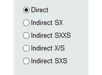 To the left of the panel we have 5 radio buttons (selectors), which will indicate to the software the form in which the input data will be entered. We will then have 5 input forms:
- Direct. By selecting this option we will be telling MCM Alchimia that we will enter the data one by one. From these data, the software will automatically obtain the mean, standard deviation of the sample means and degrees of freedom, statistics parameters necessary to perform the simulation.
- Indirect SX. This option indicates that we want the application to request two columns of data, of which each value for repeatability will be obtained from the subtraction Value = (X – S ) . An example where this option can be used is when two digital instruments are calibrated by comparison, and you want to calculate the repeatability of the errors. We indicate the reading of the pattern in the column of S and the reading of the sample in X. It can also be used when it is desired to obtain the weight of a substance contained in a crucible, through the weight of the empty crucible and with the content. In this case, the mass values of the empty crucible can be indicated in S and the mass of the crucible with the contents in X.
- Indirect SXXS. In certain cases the error values are obtained from a set of measures also known as ABBA format, which will be requested in a table of 4 columns. This format is sometimes used when it is desired to eliminate the bias caused by the potential drift of the measuring instruments. In this way, each value will be obtained from the calculation Value = (X1 + X2) / 2 – (S1 + S2) / 2 .
- Indirect X / S. In this indirect format, each value for repeats will be obtained from the Value = X / S relationship, indicated through a table of two columns.
- Indirect SXS. This format is similar to SXXS, only in three columns. The values will be obtained automatically by the application, through the operation: Value = X – (S1 + S2) / 2 .
2. Income of values.
![]() In the upper right corner of the MCM panel Alchimia has a field where we must indicate the number of repetitions to which we want to estimate the simulation parameters, that is, the mean and the standard deviation of the stockings By default the application has 10 values, however this value can be changed by manually editing the number or with the increment / decrement arrows.
In the upper right corner of the MCM panel Alchimia has a field where we must indicate the number of repetitions to which we want to estimate the simulation parameters, that is, the mean and the standard deviation of the stockings By default the application has 10 values, however this value can be changed by manually editing the number or with the increment / decrement arrows.
After indicating the number of measurements that will be entered, we click on the “Values” button, where a grid will open for the entry of values. According to the income format chosen in the radio buttons selector, the table will have the number of columns required:

3.- Simulation distribution.
 This section of the panel provides two ways to perform the simulation from the parameters of the previously defined distribution from the entered values:
Student t distribution. Selecting this option, MCM Alchimia will calculate the mean and standard deviation of the sample means from the table of values entered. Then it will generate randomized distributed according to the Student t function, with a number of degrees of freedom equal to the number of values -1.
Normal. In this case, the software will perform the same calculations as before, then take the inverse value of the function t (coverage factor k ) for the chosen coverage probability and the degrees of freedom calculated. The simulation will then be done with pseudo-randomized normal distribution of calculated mean and standard deviation s1 = ks / k ‘ , being k’ the inverse value of the distribution t for the same probability of coverage, but infinite degrees of freedom.
For a high number of degrees of freedom, both simulations will have similar or identical characteristics. In contrast, for a number of degrees of freedom <10 The results obtained from both simulations could present significant differences. Then which one to choose?
Depending on the utility that we want to give to this application, we may require one or another simulation distribution, but for technicians who are not experts in statistics, we recommend following the following rule:
- For validation of traditional calculation estimates according to GUM (JCGM 101), routine laboratory tests, proficiency tests, GUM vs MCM validation, etc. simulate according to a Normal distribution.
- For research, statistics, economics and cases where it is necessary to know accurately the impact of a variable on the uncertainty of the measurand, simulate according to a Student t distribution.
4. Forcing Mean = 0.
This option is foreseen when we want the taxpayer to whom this distribution applies only to be entered for uncertainty purposes. In this way, the average value of the function will be canceled so that the mean is = 0 and does not provide value. This is especially useful when we have model components that have more than one uncertainty, for example resolution and repeatability. In this way it can be indicated as summed variables, one constant with the value of the parameter and the rest only as contributors of uncertainty with zero value. In this case Type A can be put as experimental. The example of this help uses this tool.


