Header Image - MCM Alchimia 5

Exponential distribution

by admin 0 Comments

Exponential ditribution.

The exponential probability distribution is a continuous function in the domain of positive reals, which is suitable to represent the time between two events that are distributed according to the Poisson distribution. For example, the elapse until a trade receives its first customer of th day. The exponential distribution is a particular case of the Gamma distribution where shape parameter takes value 1.

Input parameters:

  • Mean value. This parameter must be a real number > 0 and defines the position of the mean value of the distribution. Since this is a case of the Gamma distribution, in terms of the latter, the mean would correspond to the Scale parameter if a Gamma with shape = 1 is used. In this case, the resulting probability distribution will be the same.

More help

Gamma distribution

by admin 0 Comments

Gamma distribution.

This distribution is a continuous function of biased character, that is, where the modal value does not correspond to the mean value. The Gamma distribution is a generalization of the exponential distribution, and is used in general to model random variables that represent the time in which an event occurs a certain number of times.

The pseudo-random generated by the application are an approximation (G. Marsaglia and W. Tsang) with a single input parameter called “shape”, which must be a positive real number. From version 3.2 it is possible to describe gamma functions with any standard deviation (using the second parameter named scale).

Input parameters:

  • Shape. This parameter defines the shape of the distribution. You can take as a value any number greater than zero, from field of real numbers.
  • Scale. This second parameter allows you to scale the resulting values ​​from the standard Gamma distribution, where this parameter is always 1. In this way it is possible to generate pseudo-random values with the same shape but with a greater standard deviation.

More help

Most common distribution functions

by admin 0 Comments

MCM Alchimia has a specific module for the generation of pseudo-random numbers. That is not only with classical distribution functions that allow the representation of common scenarios in risk analysis and ecomomy that contain most software of its type, but also functions used in different branches of science, covering most of the experiments developed in any analytical laboratory.

Among the most common distribution functions we can mention the following:


Tips and tricks when using MCM Alchimia

by admin 0 Comments

While MCM Alchimia can be used in any scope that requires Monte Carlo simulations, the tool has been created with the measurement uncertainty analysis in mind. This is why many of the predesigned options are unique in this software and will not be found in any similar applications (experimental distribution, analysis of calibration curves, or the result in classic GUM format according with JCGM 100). Below we detail some tips and tricks for you to become an expert in the use of the application and allow more reliable and faster results in no time.

1 .- Recommended workflow
While the application is very intuitive it is always good to follow a sequence of work to ensure both the accuracy of the calculations as well as the efficiency in the use of time. The work’s methodology can be summarized in the following stages.

  1. Definition of the mathematical model of the measurand. In this stage, the basic model (equation) of our trial is defined, just as we usually perform the calculations, or like is recommended in our reference documents.
  2. The breakdown of input quantities into sources of uncertainty. It is necessary to evaluate all the sources of uncertainty that make up each input quantity. For example, when using a measuring instrument at least two sources of uncertainty will be had, one due to calibration and another due to the resolution (or division) of the equipment. But there may also be taxpayers for additional evaluations (for instance repeatability). We recommend a Cause-Effect diagram to see in general the taxpayers of the model.
  3. Write an additional equation in subsequent rows for each magnitude of the basic model that has more than one source of uncertainty using the prefix “S” for the components that will take value = 0 and will only be included by uncertainty. This is best explained in the next item.
  4. Verify that, in each written equation, the number of parentheses opening is equal to the number of parentheses closing.
  5. It is convenient before assigning the values ​​and distributions to make a table on paper with the columns:
    Variable / Units / Value (Mean) / Probability distribution / Standar deviation (or semi-interval).
    This will allow to see each components in the generality of the model. These data will then be typed in Step 3.
  6. Following these steps will ensure success in your estimation. Remember that the use of time in your project will be 80% dedicated to the correct design of the mathematical model (the test equation).

2 .- Divide large models into several simple equations

The powerful equation editor of MCM Alchimia infinite allows you to write an unlimited number of equations in the text area. It is not necessary to write the entire mathematical model of the essay in a single line. To avoid making errors of parenthesis balance or others difficult to find at the end, it is advisable to start with a basic model that contains general variables and then write specific equations for each base quantity. You can see the example of a solved model, later in the help, which is done just in this way.

3 .- Equation editor rules

Even though is possible to represent any model with MCM Alchimia, the equation editor has some rules that it is good to remember to avoid sintax errors.

  • All equations must be written in the format [measurand] = f([variable 1],[variable 2],…,[variable n]), that is, both members of the equation must be included.
  • There can only be one magnitude of output in the model (measurand)
  • The output magnitude must be on the first line
  • It is not allowed to put “;” at the end of the line, the carriage return (enter) at the end of the line is enough to separate equations
  • It is not allowed to put two equations with the same intermediate result.
  • The editor allows ASCII characters (uppercase letters, lowercase letters, numbers and sub-characters and special characters of the virtual keyboard that can be displayed with the αβ button. Example of variable names can be “Vol_p”, “Temp2”, “δ_724”, “Δt”, etc. It is not allowed variable names like “2_t” (by number at start) or “ABS” (since it is a restricted term, it is a function)
  • Variable names must be started with an alphabetic character and moreover, numbers can not be used at the beginning of the name.
  • Variable names are case-sensitive.
  • There are reserved terms that correspond to functions, which can not be used as variable names.
  • The f(s) link on the area of ​​equations opens a keypad of functions that can be used directly in the model. If a portion of the equation is marked and then a function is selected with the keypad, this portion of the equation will remain as a parameter of the function.

4 .- How to include variables with various uncertainty contributors

A very common case in tests and calibrations is that the magnitudes have more than one source of uncertainty. For instance, the use of a measurement instrument may present several uncertainty contributions due to its calibration, resolution, repeatability, etc. To include all these sources of uncertainty, there are two ways to proceed:

  1. The magnitude can be broken down into as many addends as sources of uncertainty. The first one will take the measured or read value (as average) and the rest will be zero-centered distributions (average value = 0) since they will only be used to evaluate the uncertainty and will not influence the result. E.g. a temperature taken 10 times providing uncertainties for calibration, resolution and repeatability can be expressed as:
    T = T_cal + ST_res + ST_rep.
  2. The other option is to break down the magnitude into a constant and then the uncertainty contributors, all with average value = 0. Following the previous example would be:
    T = T_value + ST_cal + ST_res + ST_rep

Note that the variables for uncertainty, which will take zero value, were written with an initial S. While they can take any name, it is good practice to differentiate names with a common criteria like this. In this way, the structure of the model can be known already from the name of the variables.

5 .- Type A uncertainties with MCM Alchimia

A very common error in the use of the Monte Carlo method for the estimation of uncertainties is the assignment of the Normal Distribution Function to the magnitudes that present “type A” uncertainties, assigning, as standard deviation, the standard deviation of the readings.

This will yield erroneous uncertainty results (sub-estimates) due to the fact that little information about the population is taken into account, that is, the “degrees of freedom” as used in the GUM approach. By putting the calculated standard deviation directly, it is assuming that this magnitude has infinite degrees of freedom, which is not correct.

There are three ways to include correctly type A uncertainties in MCM Alchimia

  1. The JCGM 101 Evaluation of measurement data guide – Supplement 1 to the. “Guide to the expression of uncertainty in measurement” , indicates that for type A uncertainties a Student t distribution (scaled and shift) should be used, instead of a Gaussian one. For this distribution it should be indicated, as a parameter, the degrees of freedom, so that the level of information that you have of the magnitude will be included.
  2. In case you want to use the normal distribution, it can also be done, although as a standard deviation the deviation calculated in our test should be entered, multiplied by the coverage factor for our degrees of freedom and 95.45% coverage probability (inverse t distribution), divided 2. This simple operation will allow simulation taking into account the degrees of freedom of the magnitude.
  3. Our recommendation. An Exclusive specification of MCM Infinite Alchimia, is the inclusion of an FDP called Experimental. This powerful panel allows us to work with type A uncertainties directly from the raw values ​​of our test, without the need to calculate any standard deviation or other operation on our part. Using this option, the application will automatically deal with the problem of degrees of freedom, standard deviations, etc. They can even be used for more complex repeatability models, for Sample / Standard / Sample and others.

More help

First project – Results

by admin 0 Comments

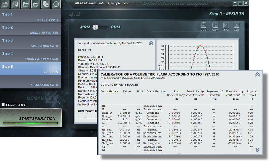
When the Start Simulation button is pressed, a bar can be seen under the button that continuously indicates the progress of random sampling. After completing the simulation with the indicated data, the application is automatically located in the results panel.

This panel shows a graphic selector at the top left, which allows to toggle between the results of the Monte Carlo simulation and the analysis according to the GUM approach, which is also estimated as well in all cases.

Next, we analyze the information provided by the MCM results view:

  1. Name of the application.
  2. Software version.
  3. Time involved by the application in obtaining results (in mm.ss, minutes and seconds)
  4. Technical data, with the text that we indicated in Step 1
  5. Number of iterations. 500 000 in our case.
  6. Statistical analysis of simulation
    1. Media = 100.04111
    2. Variance = 1.947357e-4
    3. Standard deviation = 1.39548e-2
    4. Skew = -1.01559e-3
    5. Kurtosis = 2.64392
    6. Maximum value = 100.11192
    7. Minimum value = 99,97472
    8. Median = 100.0396
    9. Range = 0.1372
  7. Normality Test (Jarque – Bera) = 2641.5964 (does not fit)
  8. Result = 100.04111. This indicates the result of the calibration without rounding figures.
  9. Confidence interval (p = 95.45%): [100.01376, 100.06841] (Half-width of the interval = 2.733e-2)
  10. Classic format: 100.041 ± 0.027 ml. This represents the test result and its associated expanded uncertainty for the coverage probability indicated in step 3. Note that this is not the result from GUM framework but the MCM results expressed as usual in GUM framework
  11. List of contributions to the uncertainty for each parameter of the model.
  12. Section with input data and mathematical model describing completely what was entered when creating the simulation project.


More help

First project – Step 3

by admin 0 Comments

Simulation data

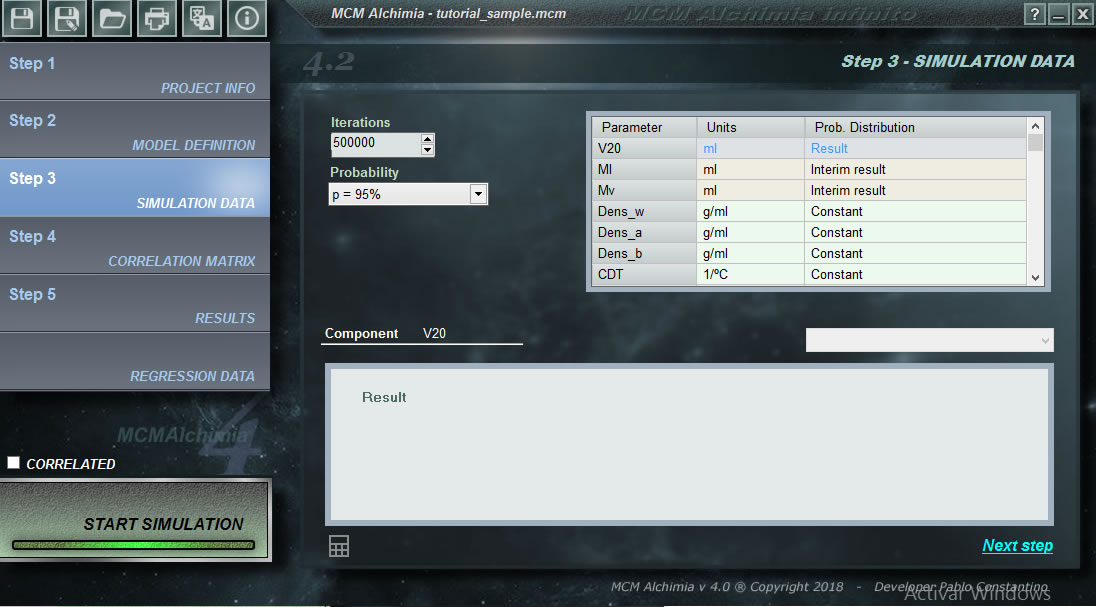
The only thing left for us to do in our first project is to assign a probability distribution function to each random variable that represents our project. As seen in the program, the grid is composed of several rows, some of them with a white background, and others with a gray background. The rows that have a gray background correspond to magnitudes for which a distribution function can not be assigned, because they are intermediate results or the final result, that is, magnitudes that will be obtained in the simulation as a result of secondary equations.

The lower part of the work panel has a command box that will give us a dropdown list of probability distribution functions so that we can select the one that fits the input magnitude. After we have selected a probability distribution, the lower box will ask us to type the necessary parameters to perform the simulation. Therefore the process of this step would be as follows:

  1. It is recommended to leave the number of iterations in 500 000 since it is obtained in excellent performance in the application and the results are absolutely reliable with this number of iterations (can be consulted the paper: Computational Aspects in the Estimation of Test Uncertainties by the Monte Carlo Method (Spanish only)
  2. We select the probability of coverage for the results. It is recommended to use 95.45% in order to obtain results for K = 2.
  3. We click on the first row with white background (or we reach it with the cursor keys of our keyboard)
  4. We select a probability distribution function in the drop-down list.
  5. We fill the simulation parameters in the lower panel (please, take units into account).
  6. We click on Apply. If everything is correct, the row will have a green background, indicating that the magnitude has its simulation data correctly assigned.

Going back to our volumetric flask we will have so:

  1. V20 : Disabled because it is Result, it is not possible to assign an PDF(Probability Distribution Function)
  2. Ml : Disabled because it is Intermediate result, It is not possible to assign a PDF
  3. Mv : Disabled because it is Intermediate result, It is not possible to assign an PDF
  4. Dens_w : We will assign the PDF Constant with a Value = 0.99829 (g / ml)
  5. Dens_a : Assign the PDF Constant with a Value = 1.2E-3 (g / ml)
  6. Dens_b : We will assign the PDF Constant with a Value = 8,000 (g / ml)
  7. CDT : Assign the PDF Constant with Value = 3.3E-6 (1 / ºC)
  8. t : Disabled because it is Intermediate result, It is not possible to assign an FDP
  9. Ml_cal : Due to an expanded uncertainty, we will assign the PDF Normal with the average value of our readings, Mean = 162,416, entering the certificate information in “Use certificate “, with uncertainty = 0.0047 (g) and k = 2
  10. SM_res : We will assign a PDF Rectangular , with Mean = 0 (corresponding to all the variables that are entered only for the purpose of estimating uncertainties) and Half interval = 0.0005 , that is, half of the division of the digital weighing scale.
  11. SM_rep : For repeatability, MCM Alchimia provides an experimental PDF where we can directly put the measured values ​​and the application will be responsible for making the statistical calculations necessary for us, to use for simulation. As it is only for uncertainty purposes we will have to select “Force Mean = 0”. We will use the “Direct” option and clicking on the Values ​​button we will enter the 5 readings of our essay: 162,384; 162,431; 162,409; 162.417; 162,439
  12. Mv_cal : Due to an expanded uncertainty, we will assign the PDF Normal with a mean in the reading of the balance in order to weigh the empty flask, Mean = 62.651, entering the certificate information in “Use certificate”, with uncertainty = 0.0047 (g) and k = 2
  13. SMv_res : We will assign a PDF Rectangular , with Media = 0 and Half interval = 0.0005.
  14. ti : Disabled because it is Intermediate result, It is not possible to assign a PDF
  15. tf : Disabled because it is Intermediate result, It is not possible to assign a PDF
  16. corr_t : We will assign the PDF Constant with Value = -0.022 (ºC)
  17. ti_cal : Because it comes from a calibration certificate, we will assign the PDF Normal with the value of our reading of the mean thermometer = 20.05. At the same time we will select “Use certificate” and we will put the expanded uncertainty = 0.021 (ºC) and k = 2.
  18. Sti_res : For this measure we use a mercury thermometer in division glass: 0.1ºC, from which we can visually estimate 1/4 of the division. According to this, we will assign a Triangular distribution with Mean = 0 and half-interval = 0.125 (this is estimate / 2)
  19. tf_cal : The same is the case as in ti_cal but now our average will be the final temperature: Mean = 20,075, select “Use certificate” and indicate the expanded uncertainty = 0.021 (ºC) and k = 2.
  20. Stf_res : Same as Sti_res, that is, Triangular with Media = 0 and semi-interval = 0.125.

When entering data for the last magnitude, the “Run the simulation” button will light up so that we can run our simulation and obtain the results. Watch results after simulation .


More help

First project – Step 2-C: Final model

by admin 0 Comments

Determination of the final mathematical model for the test.

In the previous article we saw that our flask calibration test could be represented by the following diagram;

Breaking down the input magnitudes in their contributions we would get:

  • Ml = Ml_cal + SMl_res + SMl_rep, where the suffixes “cal”, “res” and “rep” will be by calibration, instrument resolution and repeatability respectively. The prefixes “S” indicate that this component will have zero value since it is added only for the purpose of evaluation of uncertainties.
  • Mv = Mv_cal + SMv_res
  • The temperature, as we said before will be obtained from an average, so we can break down the equation in this average of readings. On the other hand, this thermometer has corrections. We could add this correction value (corr_t) to the average as a constant value without uncertainty, since this will be associated to the original values ​​of temperature.
    t = (ti + tf) / 2 + corr_t
  • but each one of these values ​​will be affected by the calibration and resolution of the thermometer. So:
    ti = ti_cal + Sti_res
    tf = tf_cal + Stf_res

Therefore to conclude this step 2:

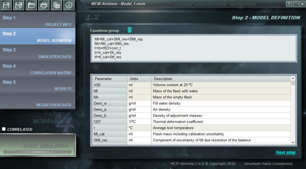
  1. We write the complete model in the text area for the Set of equations:
    V20 = ((Ml-Mv) / (Dens_w-Dens_a)) * (1- (Dens_a / Dens_b)) * (1-CDT * (t-20))
    Ml = Ml_cal + SMl_res + SMl_rep
    Mv = Mv_cal + SMv_res
    t = (ti + tf) / 2 + corr_t
    ti = ti_cal + Sti_res
    tf = tf_cal + Stf_res
  2. We fill the parameters grid with the following data:
V20
ml
Volume contained at 20 ºC
Ml
ml
Mass of the flask full with water up to calibration mark
Mv
ml
Mass of empty flask
Dens_w
g / ml
Filling water density
Dens_a
g / ml
Density of the air
Dens_b
g / ml
Density of weighing scale adjustment masses
CDT
1 / ºC
Coefficient of thermal deformation
t
ºC
Average temperature along the test
Ml_cal
ml
Flask mass including calibration uncertainty
SM_res
ml
Contribution of uncertainty of Ml due resolution of the weighing scale
SM_rep
ml
Contribution of uncertainty of Ml due repeatability
Mv_cal
ml
Empty flask mass including calibration uncertainty
SMv_res
ml
Contribution of uncertainty of Mv due resolution of the weighing scale
ti
ºC
Initial temperature of the test
tf
ºC
Final temperature of the test
corr_t
ºC
Temperature correction
ti_cal
ºC
Initial temperature with calibration uncertainty of the termometer
Sti_res
ºC
Contribution of uncertainty of ti due thermometer resolution
tf_cal
ºC
Final temperature with calibration uncertainty of the termometer
Stf_res
ºC
Contribution of uncertainty of tf due thermometer resolution


More help

First project – Step 2-B: Input uncertainties

by admin 0 Comments

Analysis of input values and their uncertainties

At this stage it is advisable to analyze the magnitudes that make up the input model to determine the contributions of uncertainty that they contribute. The advisable thing in this case is to define a model that represents as faithfully as possible the development of our analysis or trial, so that the contributions of uncertainty are adjusted to those that will really represent the model. Although we will then propose a way to do it, it is understood that each expert will do it in their own way and, therefore, the different processes will involve different final mathematical models for the trial. It is not the purpose of this aid the background discussion on volume metrology but for a given test model, finding a way to represent it faithfully.

Thus, we are assuming for our analysis that the characteristics of the test will be:

  • The flask is initially washed, dried in an oven, allowed to cool and weighed once at 20 ° C on a digital scale. This magnitude, then, will mean contributions of uncertainty for the calibration of the balance
  • The mass of the flask filled with water will be determined by repeating 5 times the measurement, weighing on a calibrated scale. Therefore this magnitude will bring uncertainty due to the calibration of the scale, its resolution and the repeatability of the measurement.
  • The temperature of the test water will be taken at the beginning and at the end of the test with a mercury glass thermometer, the average of these two measurements being used for the calculation. The contributions will then be for the calibration of the thermometer, the division thereof and for the drift found in the measurement throughout the test.
  • The other magnitudes (densities and coefficient of expansion) will be taken from tables and will be assumed constant in this opportunity (without contribution of uncertainty)

Therefore, the Cause-Effect diagram (Ishikawa) for our essay will be:

To write the complete model, then you should break down the basic magnitudes in their components, adding new lines to the model. This will be discussed in the next stage by clicking this link .


More help

First project – Step 2-A: Basic model

by admin 0 Comments

Determination of the mathematical model of the trial

In this step two we will define the mathematical model of the essay. The ISO 4787 guide details two calculation methods to obtain the volume contained in a volumetric flask. The first one indicates the calculation of the volume integrating all the magnitudes participating in the model into the equation. For a test, particularly for a defined temperature, a defined building material (glass), etc. Many of these values, such as water density and coefficient of expansion, can be considered constant, so this standard also proposes a tabulated factor to simplify the calculation. In this case we will use the complete equation to study the variables and their associated uncertainty. The equation (test model) will be:

The equation editor of MCM Alchimia is an ASCII editor that does not have special characters for which the Greek letters will have to be replaced by a common variable name. The main equation that will be put in Set equations will be V20 = ((Ml-Mv) / (Dens_w-Dens_a)) * (1- (Dens_a / Dens_b)) * (1-CDT * (t-20) ) where:

V20: Volume of the flask at 20ºC.
Ml: Mass (read on the scale) of the flask flush with detilated water (g).
Mv: Mass (read on the scale) of the empty flask (g).
Dens_w: Density of the water used in the calibration (g/ml).
Dens_a: Air density (g/ml).
Dens_b: Density of the masses with which the scale has been adjusted (g/ml).
CDT: Coefficient of cubic thermal expansion of the flask material (in 1/ºC).
t: Test water temperature (ºC).

It is advisable to make a deeper analysis of the sources of uncertainty of the input quantities of the model. In this way, if any magnitude has more than one source of uncertainty, it will be broken down into a sum of as many variables as there are sources of uncertainty, one of them will take the value of the magnitude and the rest will have zero value since they are added only for the purpose of evaluation of uncertainties.


More help