The regression panel of MCM Infinite Alchimia allows great flexibility when constructing a calibration curve for our test model.

Panel Features

1. Menu buttons In the upper left section of the panel there are three buttons that are unique to this panel.

Save. Allows you to save the data entered for the curve. This data is saved independently of the model. In this way you can use the same curve in other models and, conversely, use other calibration curves in the same model when necessary. The curves will be saved with extension .mcr.

Open curve. This button allows you to open a previously saved MCM Alchimia curve. Opening a curve does not imply that it is connected, so after opening it, you must press the connect button so that it is connected.

Clear data. Deletes all the data entered in the panel.

& nbsp;

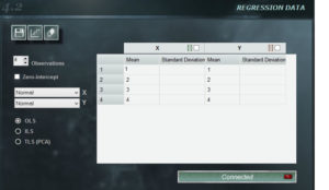
2. Number of observations. Using the forward and back buttons, the number of observations we will use to define the curve can be modified. The software offers 5 by default, but an unlimited number of observation can be indicated with a minimum of 3.

3. Intercept with zero. Selecting this option will result in an independent term = 0, regardless of the input values. In certain situations, this restriction can be defined by the knowledge of the process, for which this option is available.

4. Distribution menu. In the upper right corner of this panel are the drop-down menus where we can select probability distributions, both for the independent term, and for the dependent one. The distributions available in these combos are: Constant, Rectangular, Triangular and Normal.

If you select Constant, you are assuming that the entries on that axis have no uncertainty so the property column will be inactive and data can not be entered. In other cases, the standard deviation should be defined for the case of the normal distribution or the semi-interval for the rectangular or triangular.

5. Data panel. In this field you enter the average values ​​of x and y , as well as the properties of the distribution we choose for each axis. Important! This panel allows you to copy and paste data from any worksheet with the same form. If the copied range has larger dimensions than those indicated in the data panel, the remaining data will be truncated. The cell selected in the panel will be the upper-left cell of the copied range.

In the title cell of each axis there is a check box. Pressing this box the data of the first row of data of that axis will be copied in all the following rows.

6. Minimal square selector. In this selector we select the type of least squares method that will be used to obtain the calibration curve.

• OLS. Ordinary Least Squares. The curve obtained through this method will be the one for which the quadratic sum of the residuals in y is minimal.
• ILS. Inverse Least Squares. The curve obtained through this method will be the one for which the quadratic sum of the residuals in x is minimal.
• TLS (PCA). Total Least Squares. The curve obtained through this method will be the one for which the quadratic sum of the orthogonal residuals to the curve is minimal.

Important : This article, and therefore, the use of the tool for curves of MCM Alchimia does not take into account the assumptions related to the application of Least Squares, such as normality, linearity, homoscedasticity, and independence. The study and validation of these assumptions allow us to know the quality and applicability of the linear representation from the input data, however MCM Alchimia, allows to connect curves constructed from any input data set performing unplaced least squares and does not ensure or control compliance with these assumptions.

It is common to find trials, analytical methods or calibrations that are based on the measurement at different levels of the analyte or in different positions of the reading scale, when it is an instrument. In this way, in most cases a linear relation between them is considered, obtaining by the least squares method the coefficients of the equation of the line:

In this way when it comes to equipment calibration and the correction is plotted according to the reading scale, it is easy to obtain this value by applying the equation above, from the coefficients obtained by least squares and the reading.

But it is also usual especially in the area of ​​chemistry to construct the calibration curve with certified reference materials of known concentration and then use this curve to obtain the concentration of an analyte from an observed response.

In the least squares analysis we have three types of uncertainty associated with the curve.

• Random errors in reference responses y_i.
• Random effects on reference values ​​ x_i .
• Effect associated with the presumption of linearity, which will be given by the waste.

If the values ​​ x_i and y_i do not present uncertainty, the curve obtained will be the one that minimizes the squares of the waste. In case of random errors in reference values ​​ x_i and y_i are greater than zero, it is possible to generate pseudo-randomizations with the distribution associated to each parameter, obtaining by least squares a curve for each data set. This generates an additional uncertainty in the regression coefficients, in addition to the uncertainty determined by the residuals.

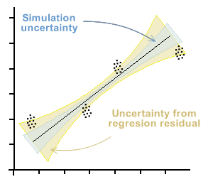
In the graph below, the beam of points that each observation would represent if there is a significant uncertainty in both axes is presented symbolically. This situation therefore yields a bundle of curves that satisfy the least squares of the residuals, generating uncertainty in both regression coefficients. This uncertainty is marked with blue in the graph.

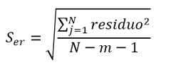
Furthermore, this uncertainty will be increased by the uncertainty inherent in the curve, which is determined as a function of the standard deviation of the residual errors. This uncertainty, in general, is greater than that of the simulation and is represented by the orange zone in the graph.

What does MCM Alchimia software do when connecting a curve?

After all the values ​​are entered into the panel, in order to use the curve in our model, we must “connect” the curve with the button provided for that purpose. When we do this, MCM Alchimia performs a simulation with the data set, performing a random sampling with the input data and the response. For each of the iterations, the regression coefficients b ₀ and b ₁ are obtained, and a value of the coefficient of determination R ² .

As in the traditional simulation, a population of data for these parameters with unknown distribution is obtained, and will depend on the distributions and values ​​of the input data.

In order not to make assumptions or inadequate approximations about these statistical properties, MCM Alchimia keeps the set of values ​​in vectors associated with these random variables, which will be available throughout the process.

On the other hand, with the average values of each pair of input data, the application calculates the uncertainty of the curve, as a function of the regression residuals.

This repository of sampling data will be used according to the need of our model, either to use the coefficients b₀ and b₁ with their uncertainty, to consider the uncertainty of the curve or to use the interpolation functions that will be described later.