 This distribution is not a distribution in itself, but a powerful and exclusive form of MCM Alchimia to enter raw values of repeatability to the model of our trial without having to make any kind of previous operations in a spreadsheet.
As can be seen in the graph, the entry data panel has several selectors to define the input characteristics of our uncertainty component.
1. Input data set
 To the left of the panel we have 5 radio buttons (selectors), which will indicate to the software the form in which the input data will be entered. We will then have 5 input forms:
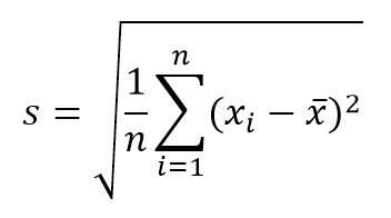
- Direct. By selecting this option we will be telling MCM Alchimia that we will enter the data one by one. From these data, the software will automatically obtain the mean, standard deviation of the sample means and degrees of freedom, statistics parameters necessary to perform the simulation.
- Indirect SX. This option indicates that we want the application to request two columns of data, of which each value for repeatability will be obtained from the subtraction Value = (X – S ) . An example where this option can be used is when two digital instruments are calibrated by comparison, and you want to calculate the repeatability of the errors. We indicate the reading of the pattern in the column of S and the reading of the sample in X. It can also be used when it is desired to obtain the weight of a substance contained in a crucible, through the weight of the empty crucible and with the content. In this case, the mass values of the empty crucible can be indicated in S and the mass of the crucible with the contents in X.
- Indirect SXXS. In certain cases the error values are obtained from a set of measures also known as ABBA format, which will be requested in a table of 4 columns. This format is sometimes used when it is desired to eliminate the bias caused by the potential drift of the measuring instruments. In this way, each value will be obtained from the calculation Value = (X1 + X2) / 2 – (S1 + S2) / 2 .
- Indirect X / S. In this indirect format, each value for repeats will be obtained from the Value = X / S relationship, indicated through a table of two columns.
- Indirect SXS. This format is similar to SXXS, only in three columns. The values will be obtained automatically by the application, through the operation: Value = X – (S1 + S2) / 2 .
2. Income of values.
 In the upper right corner of the MCM panel Alchimia has a field where we must indicate the number of repetitions to which we want to estimate the simulation parameters, that is, the mean and the standard deviation of the stockings By default the application has 10 values, however this value can be changed by manually editing the number or with the increment / decrement arrows.
After indicating the number of measurements that will be entered, we click on the “Values” button, where a grid will open for the entry of values. According to the income format chosen in the radio buttons selector, the table will have the number of columns required:

3.- Simulation distribution.
 This section of the panel provides two ways to perform the simulation from the parameters of the previously defined distribution from the entered values:
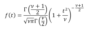
Student t distribution. Selecting this option, MCM Alchimia will calculate the mean and standard deviation of the sample means from the table of values entered. Then it will generate randomized distributed according to the Student t function, with a number of degrees of freedom equal to the number of values -1.
Normal. In this case, the software will perform the same calculations as before, then take the inverse value of the function t (coverage factor k ) for the chosen coverage probability and the degrees of freedom calculated. The simulation will then be done with pseudo-randomized normal distribution of calculated mean and standard deviation s1 = ks / k ‘ , being k’ the inverse value of the distribution t for the same probability of coverage, but infinite degrees of freedom.
For a high number of degrees of freedom, both simulations will have similar or identical characteristics. In contrast, for a number of degrees of freedom <10 The results obtained from both simulations could present significant differences.
Then which one to choose?
Depending on the utility that we want to give to this application, we may require one or another simulation distribution, but for technicians who are not experts in statistics, we recommend following the following rule:
- For validation of traditional calculation estimates according to GUM (JCGM 101), routine laboratory tests, proficiency tests, GUM vs MCM validation, etc. simulate according to a Normal distribution.
- For research, statistics, economics and cases where it is necessary to know accurately the impact of a variable on the uncertainty of the measurand, simulate according to a Student t distribution.
4. Forcing Mean = 0.
This option is foreseen when we want the taxpayer to whom this distribution applies only to be entered for uncertainty purposes. In this way, the average value of the function will be canceled so that the mean is = 0 and does not provide value. This is especially useful when we have model components that have more than one uncertainty, for example resolution and repeatability. In this way it can be indicated as summed variables, one constant with the value of the parameter and the rest only as contributors of uncertainty with zero value. In this case Type A can be put as experimental. The example of this help uses this tool.
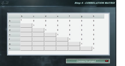 Frequently test models are used that contain two or more magnitudes with some degree of correlation, that is, that systematically, when modifying the value of one of them, the other increases or decreases. The correlation coefficients between two variables vary between -1 and 1, where the value indicates the strength of the correlation, while the sign indicates the direction. In this way, we understand that if the correlation is = 1 there is an absolute direct proportionality between the magnitudes whereas if the value is -1 the proportionality is inverse. On the other hand, a zero value for the correlation coefficient indicates that the variables are independent.


 This distribution is not a distribution in itself, but a powerful and exclusive form of MCM Alchimia to enter raw values of repeatability to the model of our trial without having to make any kind of previous operations in a spreadsheet.
 To the left of the panel we have 5 radio buttons (selectors), which will indicate to the software the form in which the input data will be entered. We will then have 5 input forms:
 This section of the panel provides two ways to perform the simulation from the parameters of the previously defined distribution from the entered values:
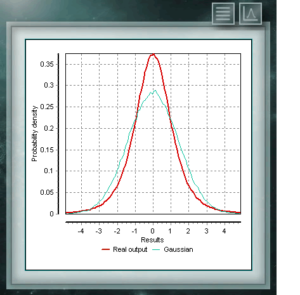 It is usual to assume in all types of analyzes, tests or calibrations, that repetitive events without external stimuli that vary their probabilities, will be distributed according to a normal or gaussian distribution defined by the mean and the standard deviation calculated for the sample. Strictly speaking this is only true when the number of repetitions is large, consistent with the central limit theorem, however when we do not have enough information to describe the properties of this gaussian distribution because our study sample is not large enough, suppose that these conditions are also fulfilled, we will surely throw values of uncertainty underestimated for our measurement, as indicated in the guide JCGM 100 – Guide to the expression of uncertainty in measurement.
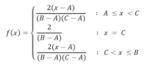
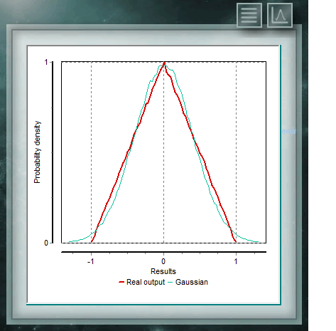 The continuous triangular distribution is characterized by being bounded to two extremes as in the case of the rectangular, but also has a mode (or value more probabe) within that range. The probability in any subinterval of equal length will increase linearly until fashion and then descend in the same way to the upper bound. This distribution is widely used in variables where information is limited, as in the case of the uniform, but where we have an approximate knowledge of the Modal value, that is, where, although the exact point of this value is not known, has information of the region or subinterval where to find it.
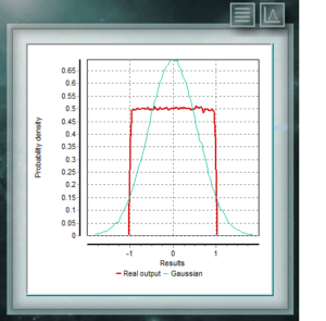 This continuous distribution is characterized by having the same probability for any value of the interval. It is widely used for contributions of type B uncertainties in which only the major and minor dimensions of the interval are known, for example in the division or resolution of a digital instrument. In many cases this distribution can also be assigned when there is little information about the random variable, in bibliographic data or when the coverage factor of an uncertainty is not known,
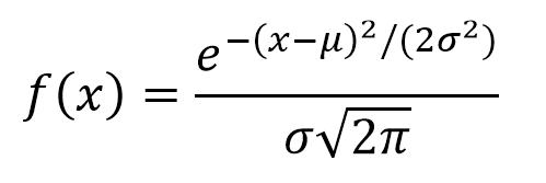
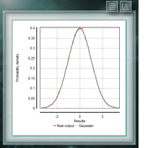 This distribution is the one that most frequently is representing natural and social events. Much of the evidence from classical statistics, as well as the estimation of uncertainties, is based on the assumption that the data conform to a normal distribution. From the theoretical perspective, the Central Limit Theorem maintains that given a random sample of sufficiently large size, it will be observed that the distribution of means follows an approximately normal distribution. The general formula of this distribution is:
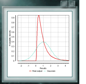 This distribution represents random variables whose logarithms are distributed according to a normal distribution. The lognormal distribution takes different forms depending on the value of its scale parameter and is often used in the reliability of high technology products and also in microbiological counts since they are based on the multiplicative growth model.
 This continuous probability distribution in the field of positive reals is intimately related to the Normal distribution, for example, it is the sample distribution of σ². The Xi (or Chi) Square distribution is defined with a single parameter which are degrees of freedom. The function is always asymmetric and biased to the right. This distribution is very frequently used in various branches of science since it allows analyzing data sets and determining if the difference between them is due to chance (null hypothesis) or to another external factor.